by Calculated Risk on 7/31/2010 10:18:00 PM

Something a little different for a Saturday evening. This is a common question, using excel, how do you get from this:

to this:I'll walk anyone interested through it (I use Excel 2007; I have 2010, but I haven't loaded it yet).

After the jump is a simple step-by-step example on one way to do it:


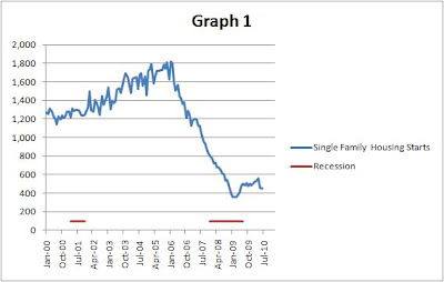
Graph 1: Start with three columns in the spreadsheet.

Here is a starter excel file (with the following data and first graph).

Set up a data file. For the example below, the first column is months, from January 2000 to January 2011 (no header), the second column uses Single Family Housing Starts from the Census Bureau, excel data here, with the column header "Single Family Housing Starts", and the third column is title "Recession" and is blank excepts for the months in recession. For the months in recession, I entered 100 (recession dates here from the NBER).

Now create a line graph by highlighting the data and clicking on insert and pick the first line graph. The result will look like this:


Graph 2: Put the recession on the 2nd axis. Do this by 1) right clicking on red recession bars, 2) Click on "Format Data Series", and 3) choose "secondary axis".


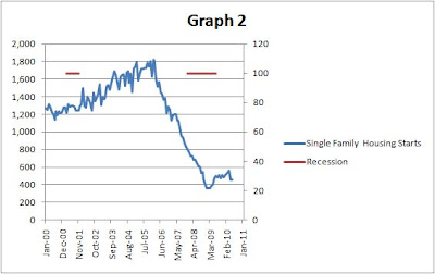
Note: It isn't necessary to put the recession on the 2nd axis and sometimes you will want to put other data there. In that case pick different numbers to mark a recession (like 2,000 instead of 100), so that the eventual columns will fill the entire range.

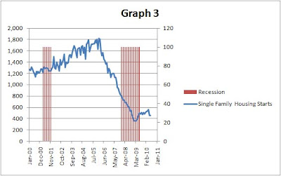
Graph 3: Change Recession from line to bars.

1) Right click on red again, 2) click on "Change Series Chart Type", 3) choose the first choice under column.

The graph now looks like:


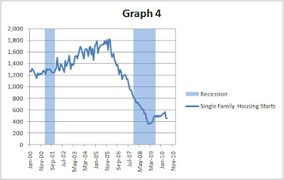
Graph 4: Some cleanup steps.

Fill the gaps and change the color.

1) Right click on red, 2) Choose "Format Data Series", 3) Change Gap Width to Zero, 4) Click on "Fill", 5) Pick "Solid fill" and color (light blue in example), 6) Change transparency to 50%.

Make columns full height and remove axis labels.

1) Right click on secondary axis labels, 2) Click on "Format Axis", 3) Change max to 100, 4) Set "axis labels" and "tick marks" to none.


Graph 5: Make it look sharp!

The final look is up to the user, but here is the look I frequently use:

Move legend to top and bold.

1) Right click on legend, 2) choose "Format legend", 3) position on "top", 4) right click on legend again, 5) increase size and bold.

Make bottom axis years. 1) Right click on horizontal axis, 2) choose "Format axis", 3) make major unit fixed at 12 months or 1 year.

Enhance single family housing starts line.

1) Right click on blue line, 2) click on "Format Data Series", 3) Choose "Line color" and red, 4) Choose "Line Style" and increase width, 5) Choose shadow and use presets "outer".

Add annual vertical grid lines.

1) Right click on horizontal axis, 2) click on "add major gridlines"

Add background to plot area.

1) Right click on plot area, 2) select "format plot area", 3) I use "Picture or texture fill" and fill with marble blue at 50% transparency.

Add title and axis labels. And you have a CR looking graph!

At this point I copy and paste the image to Photoshop (or Photoshop Elements) and sometimes make changes - and then save the file as a jpeg to upload to my blog.