by Calculated Risk on 5/25/2005 09:53:00 PM

Atlanta Federal Reserve Bank President Jack Guynn hinted at more rate hikes in his speech today. In the Q&A he commented on housing:

"There are some local markets, especially in coastal Florida, where I've heard stories for more than a year about behavior that's got to be characterized as nothing other than speculation," Guynn said it response to questions after his speech.

"It makes me very uncomfortable," he added. "Some buyers, some builders, some lenders are going to get burned, could very likely get burned, in some of those local markets."

On rates, Guynn said:

"Given the current outlook for the economy, my personal view is that we've not yet reached a neutral policy stance."

UPDATE: Dr. Polley earlier posted the same excerpts with a link to Guynn's speech.

by Calculated Risk on 5/25/2005 02:28:00 PM

On May 13, 2005 the Senate Democratic Policy Committee held a hearing on Social Security. "An Oversight Hearing on President Bush's Social Security Privatization Plan: Will You and Your Family Be Worse Off?"

There were statements from Senators and five witnesses:

Robert Shiller
Professor of Economics at Yale University

J. Bradford DeLong
Professor of Economics at the University of California-Berkeley

Derrick Max
Executive Director of the Alliance for Worker Retirement Security and the Coalition for the Modernization and Protection of America's Social Security

Peter Orszag
Senior Fellow in Economic Studies and Director of the Retirement Security Project at the Brookings Institution

Beth Kobliner
Personal Finance Columnist and Author of Get a Financial Life: Personal Finance in Your Twenties and Thirties

Many of us have read Dr. DeLong's testimony on his blog. Here is an excerpt from Dr. Shiller's testimony:

I conducted a study in March 2005 that simulates the long-term performance of personal accounts, and the paper, data and simulation program are available on my book website irrationalexuberance.com. The paper uses historical returns from 1871-2004 to assess the likely outcomes of the President’s proposal for various worker choices among the options. It does 91 different simulations for a worker born in 1990 assuming that he or she experiences the actual returns from 1871-1914, 1872-1915, 1873-1916, all the way through 1961-2004.

This sample has a U.S. historical average real stock market return of 6.8% annually, slightly above the 6.5% annual return assumed by the Social Security actuaries. My study also included “adjusted” stock market returns designed to match the median stock return in 15 countries from 1900-2000, 2.2 percentage points lower than the U.S. returns over the same time period. I believe that the international return figure is more realistic.

I found that using U.S. historical returns, a benchmark life-cycle portfolio loses money 32% of the time (i.e., 32% of the time the internal rate of return is less than the 3% real return required to break even in the proposal). The median rate of return is 3.4% annually. Using more realistic adjusted returns, the benchmark life-cycle portfolio loses money 71% of the time and has a median rate of return of 2.6%.

The conclusion is that the president’s personal accounts, even the life-cycle portfolio, would subject Americans to serious risks. The Ownership Society is a long-term and elusive goal, and we should not expose people to unnecessary risks in an overambitious attempt to attain that goal.

For those following the housing market, yes, the same Dr. Shiller.

by Calculated Risk on 5/24/2005 06:38:00 PM

According to a Census Bureau report, New Home Sales set a record in April to a seasonally adjusted annual rate of 1.316 million vs. market expectations of 1.35 million. March sales were revised down significantly to 1.313 Million.


Click on Graph for larger image.

NOTE: The graph starts at 700 thousand units per month to better show monthly variation.

Sales of new one-family houses in April 2005 were at a seasonally adjusted annual rate of 1,316,000, according to estimates released jointly today by the U.S. Census Bureau and the Department of Housing and Urban Development. This is 0.2 percent above the revised March rate of 1,313,000 and is 13.3 percent above the revised April 2004 estimate of 1,162,000.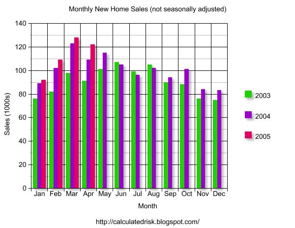



The Not Seasonally Adjusted monthly rate was 122,000 New Homes sold, down from a revised 128,000 in March.

The median sales price of new houses sold in April 2005 was $230,800; the average sales price was $283,500.

Both the median and average are in line with previous months.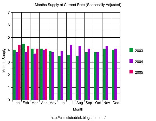



The seasonally adjusted estimate of new houses for sale at the end of April was 440,000. This represents a supply of 4.1 months at the current sales rate.

The seasonally adjusted supply of New Homes was 4.1 months, about normal for the last few years. The supply for March was also 4.1 months, revised from just 3.0 months.

The surprise was the significant downward revision in the March numbers.

by Calculated Risk on 5/24/2005 03:28:00 PM

The head cheerleader for the housing market acknowledged the housing bubble today.

"Fifteen percent price appreciation is too much, even for me," David Lereah, chief economist at the National Association of Realtors, told CNBC's "Morning Call." "The real estate market is taking on a life of its own right now and we need to get a handle on it."

Also, Equity loans alarm experts:

"If we return to prudent lending standards, that'll be the death of this housing market," says Keith Gumbinger of loan analysts HSH of Pompton Plains, N.J.

I have nothing to add to those two statements!

by Calculated Risk on 5/24/2005 12:27:00 AM

The April trade balance will be reported on June 10th. I'm trying to develop a simple model to help predict the trade deficit. Last Thursday, I posted an oil import model (I need to add exports and Seasonal Adjustments). This post will address China. I'll post my methodology and hopefully others will offer suggestions and improvements.

My general approach is to divide the deficit into two components: petroleum energy related products and everything else. This is a mixed model, by "goods" for petroleum, by country or region for everything else.

CHINA

My approach to China is to assume trade follows the normal seasonal pattern and recent growth trends. The seasonal number will be adjusted according to container traffic at the Port of Long Beach. If anything unusual has happened (change in exchange rate, labor strike, new tariffs, etc.) I will try to factor that into the estimate. For April, the only "unusual" event was the soft patch in the US economy. This probably did not impact imports, so I will assume nothing unusual for April.

US IMPORTS

First, here are the monthly imports from China for the last 6 years.



Click on graph for larger image.

Imports from China have increased every year, except in 2001 when imports were relatively flat (during the US recession). A couple of features stand out: There is a consistent seasonal pattern to imports; low early in the year, building towards the Holiday season and then dropping off at the end of the year.

The low for the year is usually in February, but it occasionally occurs in March like this year.

The second graph shows the last three years plotted against the best fit trend line. This clearly shows the seasonal pattern to imports.

Comment on Seasonal Adjustment: The seasonal adjustment is intended to remove the seasonal fluctuations from the data. This type of data is usually adjusted with a multiplicative approach: A = C x S x I where:
A = Observed Series (Not Seasonally Adjusted or NSA)
C = Trend Cycle
S = Seasonal Component
I = Irregular Component (weather, strikes, etc.)

Looking at the above graph, if the actual line is typical below the trend line for a given month, the observed numbers are adjusted upwards and if the line is usually above the trend, the oberved number is adjusted down. For April, the typical pattern shows about 4% below the trend line, so the observed number (NSA) will be adjusted upwards (SA). Errors occur if the trend changes. Also, the steeper the trend line, the more error prone the adjustment.


After reviewing the data, it appears that imports from China track inbound container shipments at the port of Long Beach. Of course this is comparing dollars to volume, so the mix of products has to remain relatively stable. The Port of Los Angeles also tracks imports relatively well, but there was a labor shortage last year and LB fit the data better.

This brings me to the first prediction for April: The trend for NSA imports for China is $17.8 Billion. Inbound container traffic was up 29% at both LB and LA ports (more than the usual March increase), so I'm going to adjust NSA upwards to $18.5 Billion.

US EXPORTS

The next step is to estimate the US exports to China. I'm going to use the same approach as for imports.


Exports to China do not show any seasonal pattern. There has been a steady increase with a slight jump in exports in 2003.

Since there is no seasonal pattern, the initial estimate is based on the trend line and the Port of Long Beach data. LB reported a 3% increase in loaded outbound containers, so the estimate will be the 3% higher than March or $3.4 Billion for April.


The final graph shows the relationship between containers and exports from LB. The bad news is the correlation is not as strong as for imports from China.

The good news is exports to China are relatively small compared to imports from China, so any error will have a minimal impact on the overall estimate.

The final step is to convert the NSA numbers to SA. Since there is little or no seasonal trend to US exports, $3.4 Billion is also the SA export number. For imports, the $18.5 Billion number is adjusted up by to $19.3 Billion.

The following table presents the actual for February and March (with estimate of the SA numbers) and the estimates for April.

CHINA TRADE BALANCE: Table numbers in Billions $
NOT SEASONALLY ADJUSTED

MONTH	NSA Balance	NSA Exports	NSA Imports
February	-$13.9	$3.08	$16.95
March	-$12.9	$3.3	$16.21
April	-$15.1(est)	$3.4(est)	$18.5(est)

SEASONALLY ADJUSTED (all estimates)

MONTH	SA Balance	SA Exports	SA Imports
February	-$18.1	$3.08	$21.19
March	-$15.1	$3.3	$18.42
April	-$15.9(est)	$3.4(est)	$19.3(est)

Note that February (usually a weak month for imports) was relatively strong and the SA number was probably over $21 Billion for imports from China, contributing to the record reported SA trade deficit.