by Calculated Risk on 6/25/2009 04:11:00 PM

A few stories too ... a major auto supplier is near bankruptcy ...

From Dow Jones: Lear Corp. Working On Prepackaged Bankruptcy - Sources

Lear Corp. (LEA), a maker of automotive seats and interior electronics, is working on a pre-packaged bankruptcy five days before it must make a $38 million interest payment on two of its bonds ... If the prepackaged bankruptcy deal falls apart, Lear could file for a traditonal-style bankruptcy next week ... The company has also lined up debtor-in-possession financing with its lenders ...

From MarketWatch: Fitch downgrades California to A-minus

Fitch Ratings downgraded the California's general obligation credit rating on Thursday to A-minus from A, based on the magnitude of the state's financial challenges and persistent weakening economy.

Click on graph for larger image in new window.

This graph is from Doug Short of dshort.com (financial planner): "Four Bad Bears".

Note that the Great Depression crash is based on the DOW; the three others are for the S&P 500.

And Jillayne Schlicke (of CEForward.com) brings us a few sample questions provided by the National Mortgage Licensing System for the new national loan originator exam: Will the New National Loan Originator Exam be Too Easy?. Here are the first two of six questions she posted:

If an applicant works 40 hours every week and is paid $13.52 per hour, what is the applicant’s monthly income?
(A) $2,163.20
(B) $2,343.47
(C) $2,379.52
(D) $2,487.68

The requirement for private mortgage insurance is generally discounted when the loan-to-value ratio falls below:
(A) 20%
(B) 50%
(C) 80%
(D) 90%

Take the test.

by Calculated Risk on 6/25/2009 03:04:00 PM

From CNBC interview (video here, comments start at 6:40) (ht Brian)

Q: You've said in some cases what appears to be a green shoot might actually end up being moss - moss growing on a rock ...

Kanas: Actually what I said is I hope it's not mold growing on a stagnant economy. But frankly I understand that there are - I hate the term green shoots, and we all talk about it every day - but I don't see it that much. I'm on main street every day, and I'm in a lot of different markets - I'm in New York half the week, and Florida half the week, and were dealing with thousands of people and hundreds of businesses every day and there are very limited green shoots from my perspective.

There is a discussion on the saving rate too and the impact on consumption. The personal income and outlays (and saving rate) for May will be released tomorrow.

by Calculated Risk on 6/25/2009 02:07:00 PM

From HotelNewsNow.com: STR posts US results for 14-20 June 2009

In year-over-year measurements, the industry’s occupancy fell 11.5 percent to end the week at 63.0 percent. Average daily rate dropped 10.1 percent to finish the week at US$96.78. Revenue per available room [RevPAR] for the week decreased 20.5 percent to finish at US$61.01.

The report also includes some hightlights on the performance for the top 25 markets. As an example, occupancy is off almost 20% in Dallas and Phoenix, and the Average daily rate (ADR) is off 30% and RevPAR off 35% in New York. Ouch.

No wonder more and more hotels are defaulting ...

Click on graph for larger image in new window.

This graph shows the YoY change in the occupancy rate (3 week trailing average).

The three week average is off 12.1% from the same period in 2008.

The average daily rate is down 10.1%, so RevPAR is off 20.5% from the same week last year.

Note: some readers might notice the occupancy rate has risen to 63% - but that is just seasonal. The hotel occupancy rate is usually the highest during the peak vacation months of June, July and August.

Data Source: Smith Travel Research, Courtesy of HotelNewsNow.com

by Calculated Risk on 6/25/2009 12:52:00 PM

From the Fed:

The Federal Reserve on Thursday announced extensions of and modifications to a number of its liquidity programs. Conditions in financial markets have improved in recent months, but market functioning in many areas remains impaired and seems likely to be strained for some time. As a consequence, to promote financial stability and support the flow of credit to households and businesses, the Federal Reserve is extending a number of facilities through early 2010. At the same time, in light of the improvement in financial conditions and reduced usage of some facilities, the Federal Reserve is trimming the size and changing the terms of some facilities.

Specifically, the Board of Governors approved extension through February 1, 2010, of the Asset-Backed Commercial Paper Money Market Mutual Fund Liquidity Facility (AMLF), the Commercial Paper Funding Facility (CPFF), the Primary Dealer Credit Facility (PDCF), and the Term Securities Lending Facility (TSLF). The expiration date for the Term Asset-Backed Securities Loan Facility (TALF) currently remains set at December 31, 2009. The Term Auction Facility (TAF) does not have a fixed expiration date.

The extension of the TSLF also required the approval of the Federal Open Market Committee (FOMC), as that facility is established under the joint authority of the Board and the FOMC.

In addition, the temporary reciprocal currency arrangements (swap lines) between the Federal Reserve and other central banks have been extended to February 1. The Federal Reserve action to extend the swap lines was taken by the FOMC.

The Federal Reserve also announced changes to certain liquidity programs in light of the improvement in financial conditions and the associated reduction in usage of some facilities. Specifically, the Federal Reserve trimmed the size of upcoming TAF auctions, because the amount of credit extended under that facility has been well below the offered amount. In view of very weak demand at TSLF Schedule 1 auctions and TSLF Options Program auctions over recent months, auctions under these programs will be suspended. The frequency of Schedule 2 TSLF auctions will be reduced to one every four weeks and the offered amount will be reduced. The authorization for the Money Market Investor Funding Facility (MMIFF) was not extended, and an additional administrative criterion was established for use of the AMLF. If necessary in view of evolving market conditions, the Federal Reserve will increase the size of TAF auctions and resume TSLF operations that have been suspended.

The TSLF lent Treasury securities to primary dealers, secured by certain other securities, for a term of 28 days rather than the usual overnight. Suspending that program seems like a minor change, but it does show the panic has subsided.

by Calculated Risk on 6/25/2009 11:00:00 AM

Earlier this week, Charles W. Calomiris, Stanley D. Longhofer and William Miles wrote in Real Time Economics that the wealth effect from housing on consumption should be small. Atif Mian and Amir Sufi of the University of Chicago Booth School of Business respond that their data indicate the opposite.

I commented on the Calomiris et. al. piece here: The Housing Wealth Effect? and I noted that Mian and Sufi disagreed.

Here are excerpts from Atif Mian and Amir Sufi's piece today:

... In the June 22nd entry for Real Time Economics, Calomiris, Longhofer, and Miles argue that ... “the reaction of consumption to housing wealth changes is probably very small.”

Findings in our research suggest the exact opposite: the rise in house prices from 2002 to 2006 was a main driver of economic growth during this time period, and the subsequent collapse of house prices is likely a main contributor to the historic consumption decline over the past year.

We agree with two key points made by Calomiris, Longhofer, and Miles. First, from the perspective of economic theory, it is not obvious that housing wealth should affect consumption. Second, it is difficult to measure the causal effect of housing wealth on consumption because other economic factors confound the relation. ...

These factors highlight the importance of quality data and sound methodology to estimate the effect of house prices on real economic activity. Our study samples 70,000 consumers in 1998 who were already homeowners at the time. We then follow the borrowing decisions of these households for eleven years until the end of 2008. Our data set represents a major advantage over prior studies; it allows us to see exactly how existing homeowners respond to increases in house prices.

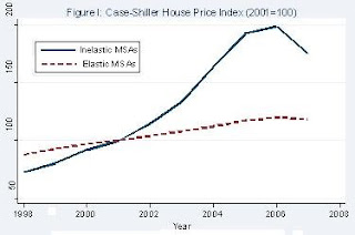
In order to isolate the effect of house prices on consumption, we rely on a simple insight: in response to an equivalent increase in local housing demand, house prices will increase more in cities where, due to geography based factors, the cost of building a house is high. For example, consider a homeowner living in San Francisco and a homeowner living in Atlanta as of 1998. From 2002 to 2006, house prices rose sharply in San Francisco where it is difficult to build additional houses because of the limited geography. In contrast, in Atlanta, where home construction is cheaper, house price growth was moderate. In economics jargon, cities where housing supply is relatively “inelastic” will experience larger movement in house prices relative to “elastic” cities (see Figure I).

Our experimental design exploits this insight in order to test how house prices affect borrowing behavior. The “treatment” group consists of homeowners in inelastic housing supply cities (e.g., San Francisco) that experienced a sharp increase and subsequent collapse of house prices. The “control” group consists of homeowners in elastic housing supply cities (e.g., Atlanta) that experienced little change in house prices.

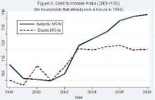
Using this methodology, we find striking results: from 2002 to 2006, homeowners borrowed $0.25 to $0.30 for every $1 increase in their home equity. Our microeconomic estimates suggest a large macroeconomic impact: withdrawals of home equity by households accounted for 2.3% of GDP each year from 2002 to 2006. Figure II illustrates the sharp increase in household leverage for homeowners living in inelastic cities.

A concern with our interpretation is that there are inherently different economic conditions in inelastic versus elastic housing supply cities that may have been responsible for the borrowing patterns we observe. However, several facts suggest that this is not a valid concern. First, inelastic cities do not experience a stronger income growth shock (i.e., a larger shock to their “permanent income”) during the housing boom. Second, the increase in debt among homeowners in high house price growth areas is concentrated in mortgage and home equity related debt.

Third, renters in inelastic areas did not experience a larger growth in their total debt. Finally, the effect of house prices on homeowner borrowing is isolated to homeowners with low credit scores and high credit card utilization rates. These “credit-constrained” households respond aggressively to house price growth, whereas the highest credit quality borrowers do not respond at all.

Our results demonstrate that homeowners in high house price areas borrowed heavily against the rise in home equity from 2002 to 2006. We also provide evidence that real outlays were a likely use of borrowed funds. Money withdrawn from home equity was not used to buy new homes, buy investment properties, or invest in financial assets. In fact, homeowners did not even use home equity withdrawals to pay down expensive credit card debt! These facts suggest that consumption and home improvement were the most likely use of borrowed funds, which is consistent with Federal Reserve survey evidence suggesting home equity extraction is used for real outlays.
...
Our analysis of the microeconomic data has led us to the conclusion that the severity of this economic downturn is rooted in the household leverage crisis, which in turn is closely related to the housing market. If the housing market continues to deteriorate, then further de-leveraging of the household sector will likely keep a lid on any rebound in consumption. In other words, the future of consumption and house prices are closely linked.

The results of Atif Mian and Amir Sufi fit with what I've observed.

by Calculated Risk on 6/25/2009 09:42:00 AM

Fed Chairman Ben Bernanke is to provide testimony before the House Committee on Oversight and Government Reform regarding the Bank of America's acquisition of Merrill Lynch. Might be interesting ...

UPDATE: Here is Bernanke's prepared testimony.

I appreciate the opportunity to discuss the Federal Reserve's role in the acquisition by the Bank of America Corporation of Merrill Lynch & Co., Inc. I believe that the Federal Reserve acted with the highest integrity throughout its discussions with Bank of America regarding that company's acquisition of Merrill Lynch. I will attempt in this testimony to respond to some of the questions that have been raised.

Here is the CNBC feed.

And a live feed from C-SPAN.

by Calculated Risk on 6/25/2009 08:30:00 AM

The DOL reports on weekly unemployment insurance claims:

In the week ending June 20, the advance figure for seasonally adjusted initial claims was 627,000, an increase of 15,000 from the previous week's revised figure of 612,000. The 4-week moving average was 617,250, an increase of 500 from the previous week's revised average of 616,750.
...
The advance number for seasonally adjusted insured unemployment during the week ending June 13 was 6,738,000, an increase of 29,000 from the preceding week's revised level of 6,709,000. The 4-week moving average was 6,759,750, a decrease of 3,250 from the preceding week's revised average of 6,763,000.

Click on graph for larger image in new window.

This graph shows weekly claims and continued claims since 1971.

Continued claims decreased to 6.74 million. This is 5.0% of covered employment.

Note: continued claims peaked at 5.4% of covered employment in 1982 and 7.0% in 1975.

The four-week average of weekly unemployment claims increased this week by 500, and is now 41,500 below the peak of 10 weeks ago. There is a reasonable chance that claims have peaked for this cycle.

However the level of initial claims (over 627 thousand) is still very high, indicating significant weakness in the job market.

There was plenty of discussion about the decline in continuing claims last week. A few comments:

My view is the most useful number in the weekly claims report is the number of seasonally adjusted initial claims (with a 4-week moving average because it is so noisy). This has declined from the peak of 10 weeks ago, but is still very high. This suggests that the peak of job losses might be behind us, but also that there are still significant job losses occurring. We will probably see monthly job losses reported by the BLS until the weekly initial claims numbers declines close to 400 thousand.

The continuing claims number can decline for several reasons: 1) some pickup in hiring, 2) standard unemployment benefits may be expiring, and 3) the estimate might be revised. The continued claims estimate for last week was revised up some - so that explains part of it. Also, as people move off the standard 26 week unemployment benefits, they are no longer included in continued claims (for the most part). These people are still receiving extended benefits, but that is tracked elsewhere.

If we look back 26 weeks from last week, there was a huge jump in NSA initial claims (from 536 thousand to 760 thousand) or 224 thousand in one week back in December. Any of those people who are still unemployed (and many probably are) were moving off the standard unemployment benefits to extended benefits and are no longer counted in the continued claims. That probably counts for most of the decline last week. But it is also important to remember they are still receiving unemployment benefits (extended benefits).

When looking at this report, I'd focus on the 4-week moving average of initial claims, not continued claims.

by Calculated Risk on 6/24/2009 11:31:00 PM

Here is the CRE report mentioned yesterday, from RC Analytics: Moody’s/REAL Commercial Property Price Indices, June 2009

The Moody’s/REAL National All Property Type Aggregate Index for April measures 135.31, a decrease of 8.6% from the previous month. The index now stands 25.3% below the level seen a year ago and 29.5% below the peak measured in October 2007. The index is 27.4% lower than it was two years ago. This report is based on data through the end of April.
...
The Moody’s/REAL Commercial Property Price Indices (CPPI) measure the change in actual transaction prices for commercial real estate assets based on the repeat sales of the same assets at different points in time. ... A summary or short version of the repeat sales methodology is available in a Moody’s Special Report. US CMBS: Moody’s Publishes the First Commercial Property Price Indices Based on Commercial Real Estate Repeat Sales Data. Sept. 19, 2007. This is available on Moodys.com > Structured Finance > Commercial MBS > CRE Indices. A very detailed and complete explanation of the methodology is available in a White Paper from MIT. David Geltner and Henry Pollakowski. A Set of Indexes for Trading Commercial Real Estate Based on the Real Capital Analytics Transaction Prices Database. MIT Center for Real Estate. Sept. 26, 2007.

Note that the Moody's CRE price index is a repeat sales index like Case-Shiller.

Click on graph for larger image in new window.

Here is figure 1 from the report. CRE prices are back to 2004.

The Case-Shiller Composite 20 residential index is added in red (with Dec 2000 set to 100).

This shows residential leading CRE (although we usually talk about residential investment leading CRE investment, but in this case also for prices), and this also shows that prices tend to fall faster for CRE than for residential.

by Calculated Risk on 6/24/2009 08:51:00 PM

Earlier today I posted some analysis of the gap between existing and new home sales: Distressing Gap: Ratio of Existing to New Home Sales (see the post for several graphs - including the ratio between new and existing home sales)

Professor Brian Peterson has more (including some thoughts prices): House Prices and New versus Existing Homes Sales

To get a feel for how the two series [New and existing home sales] move together, figure 2 plots the percentage deviation for each series from its mean from 1975-2008. We see clearly that from 1975 to 2006 (the solid lines) that new home sales and existing homes sales move around together, with a correlation of 0.944 over the the time period up to 2006. However, as shown by the dashed lines, a gap has developed post 2006, resulting in the correlation for the sample from 1975-2008 falling to 0.876. There seems to be some type of a shock that is driving existing homes sale up relative to new homes sales.

I find it strange that most analysts are looking at existing home sales for stability in the housing market. I think the new home market is the place to look.

by Calculated Risk on 6/24/2009 07:46:00 PM

From Bloomberg: King Says U.K. Recovery May Be ‘Long, Hard Slog’ (ht Jonathan)

“There has to be a risk that it will be a long, hard slog” because of the problems in the banking system, King told lawmakers in London today. “I feel more uncertain now than ever. This is not the pattern of a recession coming into recovery that we’ve seen since the 1930s. Having an open mind and not pretending to foresee the future when it’s so uncertain is important.”
...
King said that there’s “not much evidence to change our view” since the bank released forecasts in May showing that the economy won’t return to growth on an annual basis until the second half of next year.
emphasis added